Deployment: Detection
One of the biggest challenges for automated insect monitoring by running model inference on devices with relatively low computational power, is to find the right balance between speed (fps) and accuracy of the detection and classification results. A high speed or image throughput is necessary for the object tracker to work correctly, as it depends on the information (bounding box coordinates) coming from the detection model. If the speed (fps) of the model output is too low, fast moving insects can not be properly tracked, which will lead to "jumping" tracking IDs and thereby multiple counting of a single individual.
Model speed can be increased by choosing small models with fewer parameters (e.g. YOLOv5n) and decreasing the resolution of frames that are used as input for the model (e.g. 320x320 pixel). However, the reduced image resolution can significantly decrease the detection and especially classification accuracy. This effect is even stronger when dealing with very small objects like insects.
A possible solution to this problem could be to use a smaller field of view (FOV), e.g. by using a small flower platform and short distance between platform and camera. This would however decrease the efficiency of the visual attraction and fewer insects could be recorded in the same time frame. In the following, an alternative approach to this problem is proposed.
Processing pipeline
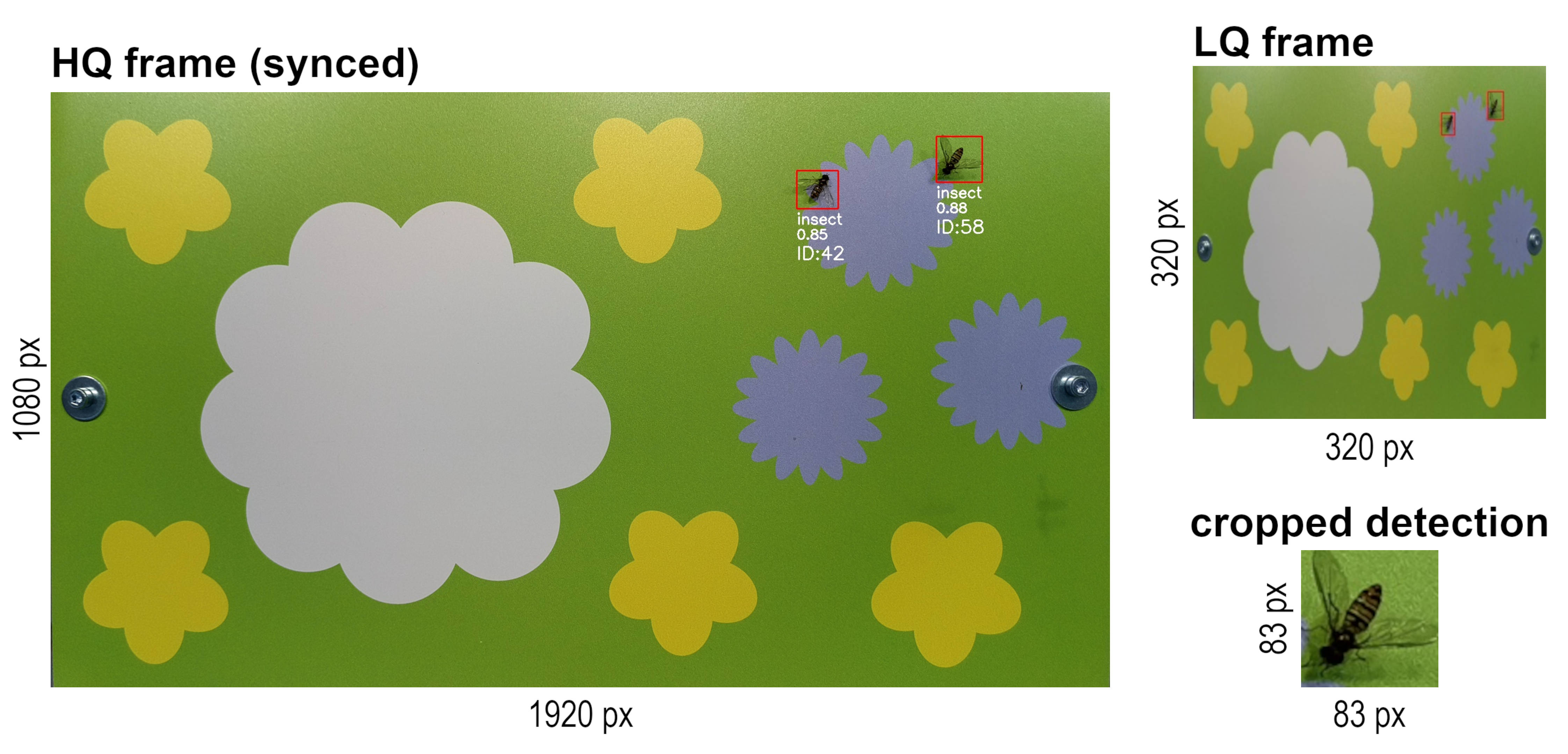
The OAK-1 camera and DepthAI Python API make it possible to run a low-quality (LQ) stream (e.g. 320x320 px) in parallel with a high-quality (HQ) stream (e.g. 3840 x 2160 px) and synchronize the detections made on the LQ stream with the frames from the HQ stream on-device. This approach enables the use of the LQ stream as input for a YOLO detection model to increase the possible inference speed, which in turn also increases the performance and accuracy of the object tracker.
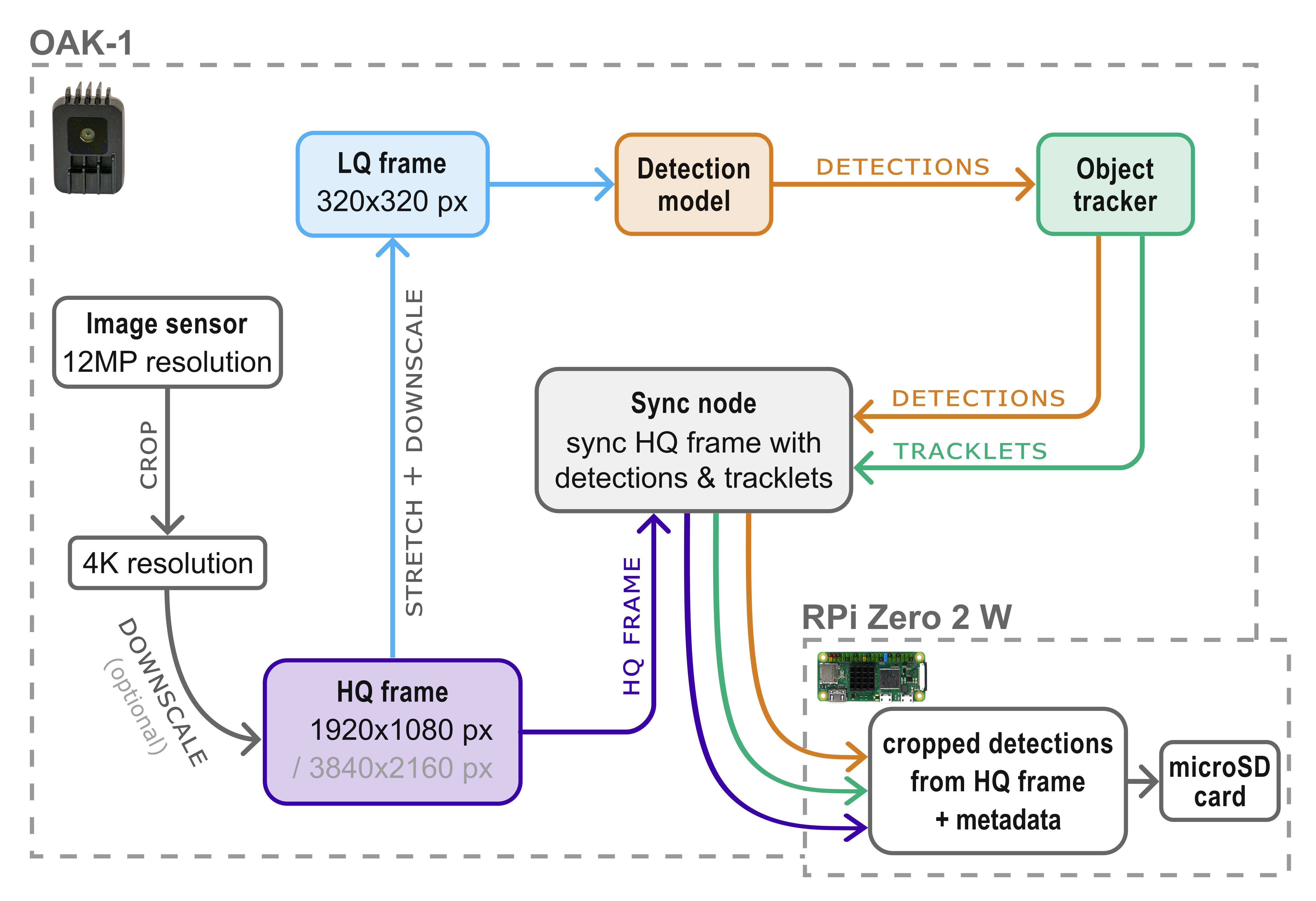
As the insects in these LQ frames often miss visual features that would be important for a good classification accuracy, it is recommended to use only one generic class ("insect") for the detection model training and inference. To still be able to classify the detected insects in a subsequent step, the detections (= bounding box coordinates) and tracklets (= tracking ID) are synchronized with the HQ stream in real time on-device. In this way it is possible to crop the detected insects (area of the bounding box) from the HQ frames and save them as individual .jpg files (e.g. every second). The cropped detections have a high enough resolution for accurate classification in a subsequent step on your local PC.
Separating the detection and classification steps can also simplify dataset management, annotation and model training. Overall less training data is sufficient for good detection results, as no classes have to be distinguished by the detection model. You can directly use the cropped detections as input for a growing image dataset to train new insect classification models, just by sorting them to folders with the respective class name (e.g. insect taxon).
Metadata .csv
For each cropped detection that is saved to .jpg, a new row with relevant metadata is appended to a metadata .csv file that is created for each recording event. This metadata includes:
rec_ID, calculated with the number of already existing recording folders to distinguish each recording event. This is important, as the unique tracking IDs will restart from 1 for each recording interval and the metadata .csv files will be merged during the automated classification step.timestampwith exact recording time.labelis negligible if a detection model with only one class is used, but enables the deployment of a multi-class detection model.confidencescore can be used to evaluate the quality of the detection results, e.g. to find examples where the model is uncertain or to filter only detections above a specific confidence score threshold.track_IDthat is assigned by the object tracker node to each individual insect. As cropped detections are saved in short time intervals (e.g. every second), many images can exist of an individual tracked insect, dependent on its duration of stay on the flower platform. All of these images are classified in the next step and the class with the highest weighted probability is then calculated in the final step by using theprocess_metadata.pyscript.x_min,y_min,x_max,y_maxrelative bounding box coordinates. These coordinates make it possible to calculate the relative bounding box size. If the absolute frame dimensions (e.g. size of the flower platform in mm) are used as argument for theprocess_metadata.pyscript, the absolute average bounding box size in mm is calculated for each detection.file_pathto the cropped detection, saved as .jpg.
| rec_ID | timestamp | label | confidence | track_ID | x_min | y_min | x_max | y_max | file_path |
|---|---|---|---|---|---|---|---|---|---|
| 1 | 20221201_16-41-02.393074 | insect | 0.87 | 1 | 0.5647 | 0.5357 | 0.6321 | 0.6132 | ./insect-detect/data/20221201/20221201_16-40/cropped/insect/20221201_16-41-02.393074_1_cropped.jpg |